This article explores the variety of setups and methodologies involved in testing antennas and antenna arrays, including far-field test ranges, near-field test ranges, and phased-array systems.
Understanding Antenna Measurements
Antenna performance is crucial to every system. Antenna gain is a key variable in the radar range equation (see Sidebar) and therefore directly affects range.
The gain value is defined as the maximum power relative to the power emanating from an isotropic antenna (i.e., a point source). Gain is usually defined in logarithmic terms, namely dBi, which indicates dB relative to an isotropic antenna. It is expressed with the following equation:
Where:
h = antenna efficiency
A = antenna area
λ = wavelength of the carrier signal in meters
In addition to gain, polarization is another important consideration for antennas: the polarizations of the transmit and receive antennas must match to ensure efficient signal transfer. Types of polarization include linear (vertical or horizontal), and circular. Elliptical polarization (or ellipticity) is a measure of deviation from desired linear or circular polarization.
Antenna patterns are used to illustrate and quantify how an antenna radiates energy versus angular direction. Various parameters of an antenna can be determined from an antenna pattern (Figure 1).
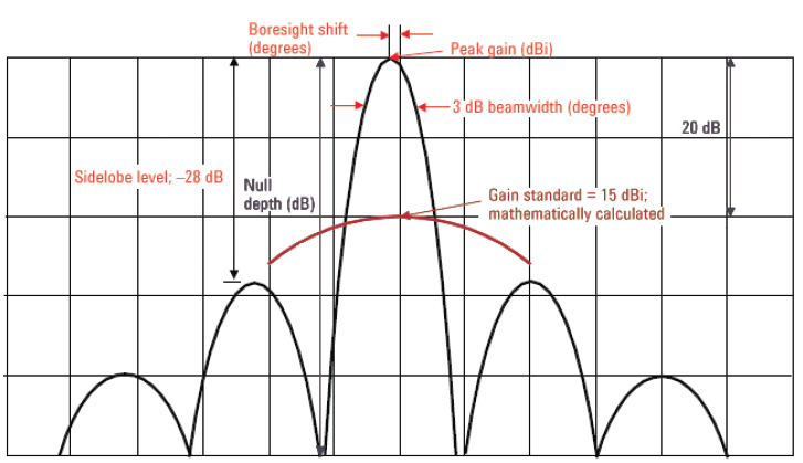
Figure 1. An antenna pattern characterizes how an antenna radiates electromagnetic energy versus angular position. Antenna pattern characteristics can also be determined.
An antenna’s beamwidth is not necessarily the same horizontally and vertically. For example, a tracking antenna may have a “pencil” beam that is of equal width in the horizontal and vertical directions, while a search antenna may have a fan-shaped beam that is narrow in the horizontal and wide in the vertical. Beamwidth and antenna gain are interrelated; as the beamwidth is narrowed, the gain increases because the radiated energy is more focused.
Legacy radar antennas relied on mechanical positioning systems to steer the beam. Many current generation systems use active electronically scanned arrays (AESA) to scan or steer the beam. These AESA antennas, or phased array antennas are made up of hundreds to thousands of individual radiating elements whose phase and amplitude can be independently controlled and changed rapidly with each pulse that is radiated by the radar. AESA antennas are becoming quite popular due to their faster steering and scanning capability, which allows multiple targets across wide areas to be tracked simultaneously and accurately.
Sidelobes are an undesirable artifact of beam forming. Because sidelobes transmit energy in unwanted directions, they can produce false returns from objects close to the antenna, which is why they should be kept as small as possible. Although sidelobes are generally small, they can be measured against theoretical limits for a specific type of antenna design.
Input impedance of an antenna is an important parameter to measure, since it affects the efficiency of an antenna. Power that is reflected from the input connector of an antenna is not available to be radiated. A network analyzer is usually used to measure input impedance, and is typically expressed in VSWR, reflection coefficient, or return loss.
Far-field and Near-field Ranges
A radiating antenna has three radiating regions (as shown in figure 2 left). The reactive region extends from the surface of the antenna to (for electromagnetically short antennas that are less than λ/2 in length, we use R = λ/2π = 0.159λ). The radiative region extends from to a generally accepted transition to the ‘far-field’ at 2D2/λ.
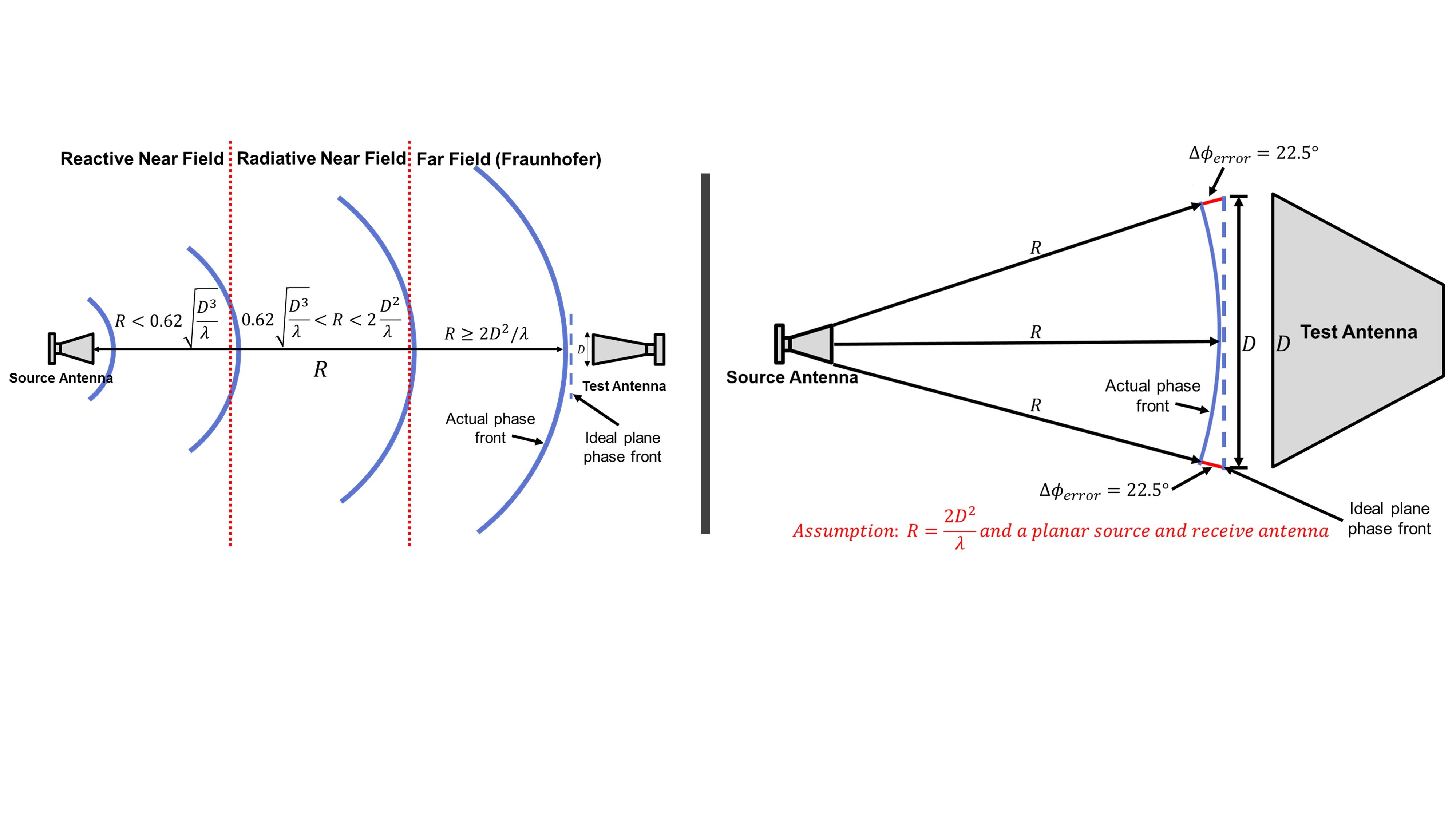
Figure 2: The Near and Far Field Criteria (left). Zoom view showing 22.5° phase deviation when R=(2D^2)/λ (right).
The Radar Range Equation
Here is the simplified version of the radar range equation expressed in log form (dB):
40 log(Rmax) = Pt + 2G + 20 logλ + σ + Ei(n) + 204 dBW/Hz – 10 log(Bn) – Fn – (S/N) – Lt – Lr – 33 dB
Where:
- Rmax = maximum distance in meters
- Pt = transmit power in dBW
- G = antenna gain in dB
- λ = wavelength of the radar signal in meters
- σ = RCS of target measured in dBsm or dB relative to a square meter
- Fn = noise figure (noise factor converted to dB)
- S/N = minimum signal-to-noise ratio required by receiver processing functions to detect the signal in dB
The 33 dB term comes from 10 log(4π)3, which can also be written as 30 log (4p), and the 204 dBW/Hz is from Johnson noise at room temperature. The decibel term for RCS (σ) is expressed in dBsm or decibels relative to a one-meter section of a sphere (e.g., one with cross section of a square meter), which is the standard target for RCS measurements. For multiple-antenna radars, the maximum range grows in proportion to the number of elements, assuming equal performance from each one.
Far-field Range Testing
Since antennas are operated at a long distance from each other, a spherically radiated wave looks almost planar when received by the antenna under test. A far-field antenna range attempts to simulate a planar wavefront by locating the AUT a long distance from the source antenna which also radiates a spherical wavefront. (Refer to Figure 2 – right). The long distance allows the spherical radiated wavefronts to become nearly planar by the time they reach the AUT. The generally accepted far-field range criteria is ,where D is the aperture diameter of the antenna under test and λ is the wavelength. At a range distance of 2D2/λ, there is 22.5 degrees of phase taper across the aperture of the antenna, and this causes some measurement inaccuracies of the sidelobe levels. During a far-field measurement, the amplitude response of the AUT is measured in real time as the AUT is rotated through a range of azimuth and elevation coordinates. The rotation of the antenna is accomplished with a mechanical positioner that moves the AUT in a single axis at a time, and provides position feedback to the measurement system.
While far-field measurements have been widely used for many years, they have some disadvantages. Depending on the size of the antenna and the frequency, the range length can be quite long, resulting in large dispersive losses. Far-field ranges are more susceptible to reflections, and if the range is located outdoors, weather and security (visual & frequencies) are a concern. Typically, a far-field range takes much longer to fully characterize an antenna due to the relatively slow positioner velocity, and the need to rotate the AUT through many different angular scans. Measurement software can be used to carry out the normally laborious process of controlling the antenna position and synchronizing the source and network analyzer during each measurement. For a larger far-field antenna range, controlling a remote source across a significant distance can be problematic.
Near-field Range Testing
Because of the many disadvantages of far-field antenna ranges, the near-field testing technique has become quite popular over the past 25 years. Near-field ranges require much less space, protect antennas from weather, provide better security, and do not have any phase taper. This technique does require a lot of computations, but with the power of today’s PCs, this is no longer a concern.
A near-field measurement technique (for measuring the far-field antenna pattern) samples the amplitude and phase radiated by the AUT at λ/2 grid points across the radiating aperture of the antenna. Once all significant energy has been sampled, a 2 or 3-dimensional Fourier Transform is used to compute the far-field antenna radiation patterns. While near-field probing can occur anywhere in the radiative region, typically the distance between the probe antenna and the AUT is 1λ-3λ, thus the dispersive loss is much less, and the signal-to-noise ratio is much higher, and there is also processing gain from all the sample points.
The challenge of a near-field measurement is to sample the amplitude and phase at precise λ/2 grid points. To do this requires a precision mechanical scanner to move the probe antenna to capture all the significant radiated energy. Depending on the type of antenna radiation pattern, there are three different near-field scan types, planar, cylindrical, or spherical.
Once all the significant energy has been sampled, this data set contains all the data to completely characterize the AUTs’ radiation patterns. Modern near-field software programs can display an antenna’s radiation patterns in a variety of visual formats. One trade-off from the near-field measurement technique is that all the data points need to be sampled before a single principle plane antenna pattern can be displayed.
Example measurements
Figure 3 shows two example measurement results. The plot on the left shows a far-field antenna pattern in the horizontal plane. Measurement results from the principal planes provide a lot of information about the performance of the antenna, and are often used to characterize antenna performance—gain, beam width, sidelobe level, etc.
The plot on the right shows the co- and cross-polarization response of an antenna. The co-polarized response is the desired polarization response of the AUT, and the cross-polarized response is the undesired polarization response.
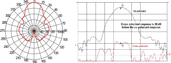
Figure 3. These examples show a horizontal-plane antenna pattern (left) and cross polarization in an antenna pattern (right).