In Digital modulation basics, part 1 we examined the concept of quadrature modulation and signal generation. We showed a common block diagram for generating a quadrature signal (Figure 1). There is a corresponding receiver block diagram to extract the Inphase (I) and Quadrature (Q) components of the signal (Figure 2). The signal is converted to digital form by the analog-to-digital converter (ADC) and then processed using digital techniques. It doesn’t have to be this way—the system can be implemented using analog circuits—but most quadrature receivers are digital.
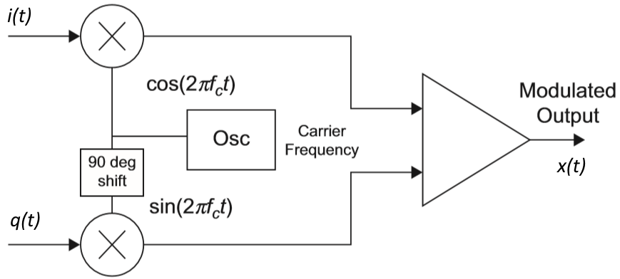
Figure 1. A quadrature modulator produces a modulated output by combining two modulated carriers: the inphase portion, i(t) and the quadrature portion, q(t). The quadrature carrier is shifted by 90 degrees.
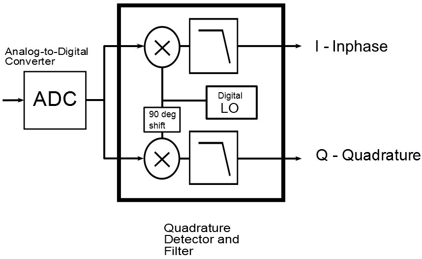
Figure 2. A quadrature receiver takes the digitized component signal and separates it into the original Inphase and Quadrature data streams.
The I signal is created by multiplying the incoming signal by the digital local oscillator (LO). The resulting signal goes through a lowpass filter to remove higher-frequency products, creating the I signal, still in digital form. The Q path operates the same way but with a 90-degree phase shift applied to the LO. At the output, we have two data streams, commonly referred to as the I/Q data for the received signal.
Error Vector Magnitude
The function of the receiver is to extract the vector information from the signal, which can be expressed in amplitude/phase or I/Q form, as shown in Figure 3. Real-world signals have noise and other imperfections that compromise the ability of the receiver to demodulate the signal and recover the transmitted bits. The communications industry uses the concept of Error Vector Magnitude (EVM) to describe the error in a quadrature-modulated signal. EVM is sometimes called Relative Constellation Error (RCE).
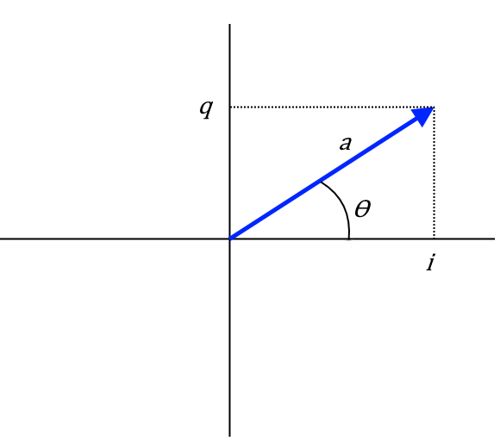
Figure 3. The vector representation of a quadrature signal.
As shown in Figure 4, the Error Vector represents the vector difference between the measured signal and an ideal version of it. EVM is the root-mean-square (RMS) value of the error vector over some time interval (evaluated at the valid symbol times). EVM is normally reported as a percent of the ideal signal but may be shown in decibel form. The ideal signal may be defined as the square root of the mean power of the ideal signal, the average symbol power, or the peak signal level.
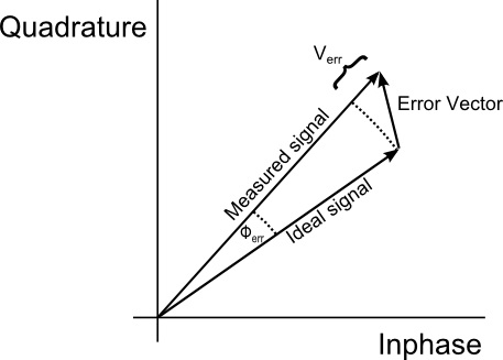
Figure 4. Error Vector Magnitude (EVM) is the magnitude of the error vector, drawn from the ideal signal to the measured signal.
Measuring EVM requires an accurate receiver that can compare the measured signal to an ideal version of it. With today’s complex modulation formats, the measurement receiver must be aware of the specific modulation format being used, performing the EVM measurement only during the valid symbol times.
Constellation Diagram
Figure 5 shows the constellation diagram for a 16-QAM signal. Each of these 16 vector states represent 4 bits of information. Ideally, these states would be tiny points on the diagram, with no noise or distortion present. Of course, communication channels are always imperfect so a real signal will be spread out on this display. Broadband noise, phase noise, non-linearities, frequency response errors, and interfering signals can all contribute to a degraded EVM.
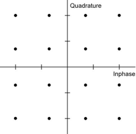
Figure 5. 16-QAM Modulation uses 16 combinations of amplitude and phase to represent four bits (16 combinations).
Figure 6 shows a measurement of a 16-QAM signal. The window on the left shows the dot associated with each vector state, surrounded by a circular error limit. Vectors that land inside the error limit are considered “good” while the ones outside of the limit are “bad.” The signal shown is very clean with all the dots inside the error limits, and the EVM is 0.37%.
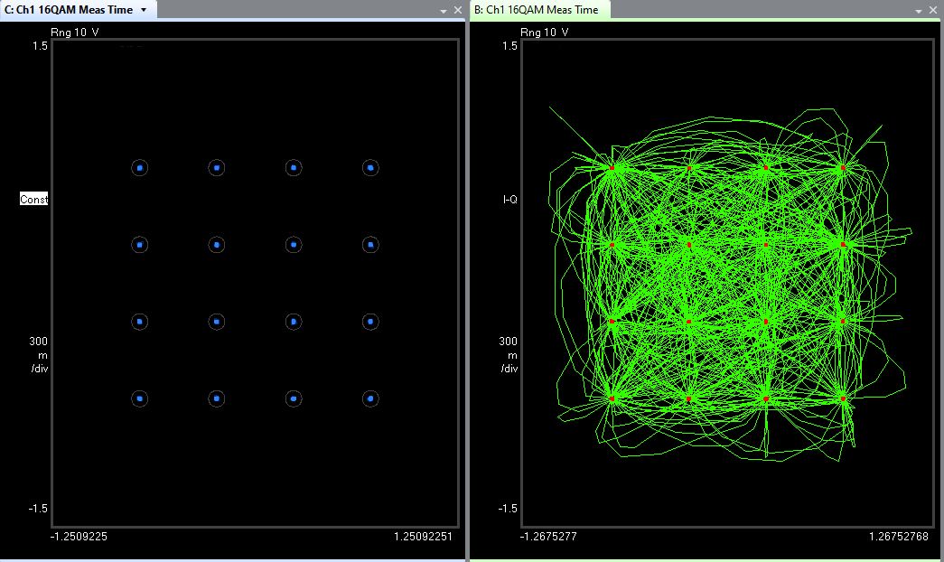
Figure 6. The constellation diagram of a 16-QAM signal with an EVM of 0.37%, as measured with Keysight Technologies PathWave Vector Signal Analysis software.
In the left window, the vector state is only displayed at the valid sample window of the vector. On the right window, however, the time between valid states are also shown such that we can observe the vector transitions. This can be important information to understand the system performance and troubleshoot why the system is experiencing errors.
Figure 7 shows a degraded 16-QAM signal, having an EVM of 10.0%. On the left window of the figure, we see that the constellation dots are much more random and spread out. This is consistent with a degraded EVM and increased digital errors in the received signal.
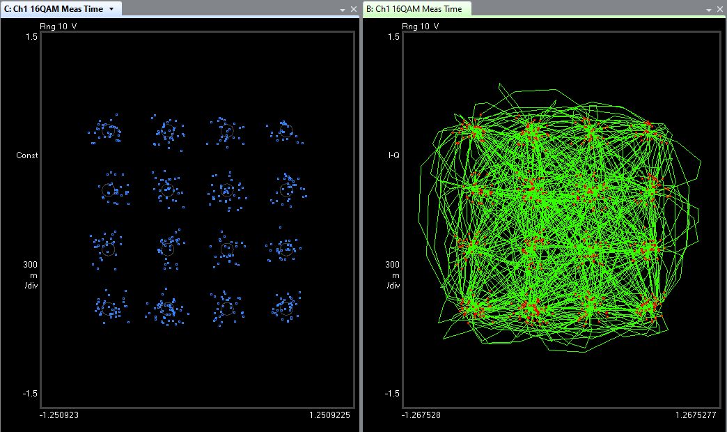
Figure 7. The constellation diagram of a 16-QAM signal with errors in the signal, resulting in an EVM of 10.0%.
Another useful measure of the system performance is to count how many bits are recovered incorrectly. The standard measure for this is the bit-error ratio (BER), defined as the number of bit errors divided by the total number of bits transferred during a specific time interval. Larger EVM values correspond to larger BER.
The 16-QAM modulation discussed here is relatively simple and easy to view. However, higher-order QAM systems such as 64-QAM, 256-QAM and 1024-QAM are often used to obtain higher system throughput. Early 5G designs are using 256-QAM, which requires an EVM of 3.5%. Future designs will incorporate 1024-QAM.
References
- Spectrum and Network Measurements (2nd Edition), Section 6.12 Quadrature Modulation, Robert A. Witte, SciTech Publishing, 2014.
- “Digital Modulation in Communications Systems- An Introduction,” Application Note, Publication Number 5964-7160E, Keysight Technologies, 2014. http://literature.cdn.keysight.com/litweb/pdf/5965-7160E.pdf
- “8 Hints for Making and Interpreting EVM Measurements,” Application Note, Publication Number 5989-3144EN, Keysight Technologies, 2017. https://www.keysight.com/us/en/assets/7018-01305/application-notes/5989-3144.pdf.
- Cavazos, Jessy, “Overcoming 5G NR mmWave Signal Quality Challenges,” Keysight Technologies, 2019. https://blogs.keysight.com/blogs/inds.entry.html/2019/09/30/overcoming_5g_nrmmw-4xyP.html
Related articles
- Digital modulation basics, part 1
- Measuring phase noise and jitter
- How standards and conformance tests shape the future of 5G New Radio
- Examining Common Smartphone WiFi Quality Issues And How WiFi Performance Testing Can Help
- Precision and accuracy in oscilloscopes
 Bob Witte is President of Signal Blue LLC, a technology consulting company. Bob has held many positions in R&D, technology planning, strategic planning, and manufacturing for Keysight Technologies, Agilent Technologies and Hewlett-Packard Company. Inside, he is just an engineer that loves to see innovative products solve real customer problems. Bob is the author of two books on test and measurement instrumentation: Electronic Test Instruments (2nd Edition) and Spectrum and Network Measurements (2nd Edition).

Tell Us What You Think!